AmPtool

AmPtool
contains Matlab functions for the visualisation and analysis of patterns in (functions of) parameter values of the
Add-my-Pet (AmP) collection.
We will hereafter refer to functions of DEB parameters as "traits", be they at individual or population level.
The AmPtool GitHub repository itself does not contain data,
and is designed as an add-on for the free open-source package of DEB functions for Matlab, DEBtool_M.
Moreover, AmPtool must access the data behind the AmP collection.
Said data is available via the AmP website.
Simply access the website, click on the dropdown menu COLLECTION and then select AmPdata.
Please see here below a screen shot of the AmP webpage menu for a visual on how to download the data from the collection.
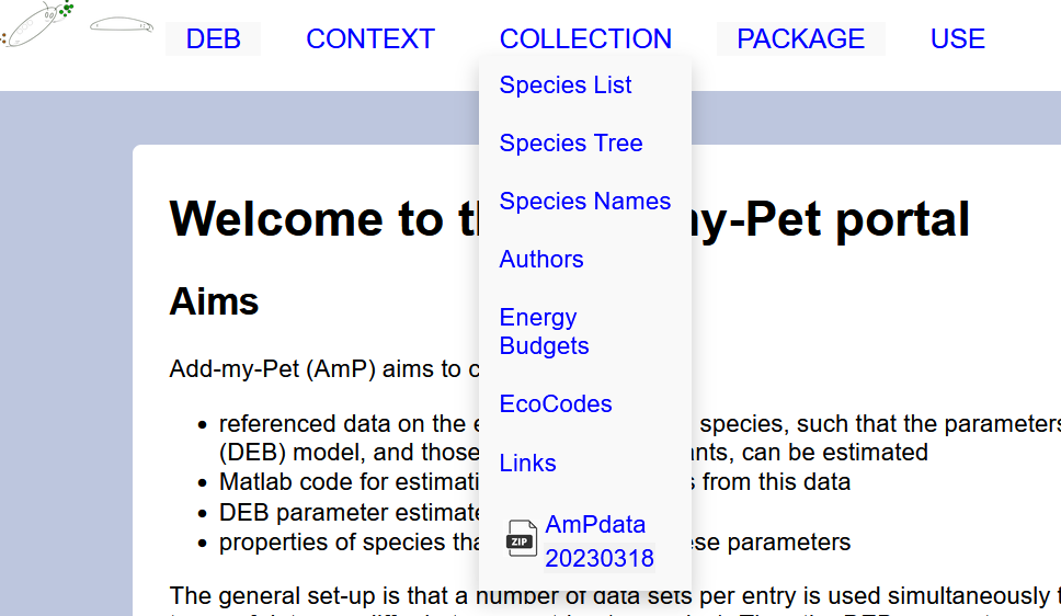 Notice that the date the data was written into the AmPdata files is specified.
AmPdata is stored as a zip-file which when you extract locally on your device contains four files:
Notice that the date the data was written into the AmPdata files is specified.
AmPdata is stored as a zip-file which when you extract locally on your device contains four files:
allStat.mat(all parameters at reference temperature, and traits at body temperature for each animal in AmP are stored herein)popStat.mat(population level traits at body temperature for each animal in AmP are stored herein)allUnits.mat(units for each parameter and trait are stored herein)allLabel.mat(desciption of each parameter and trait are stored herein)
.mat files (which we name AmPdata but you are free to chose the name that works for you).
Make sure to work with the latest versions since all of the AmP species which are found in .txt files stored AmPtool/taxa should correspond exactly with AmPdata and they both change frequently.
One way to make sure that the AmPdata stored locally on you PC and to which you set a Matlab path matches the latest version which is on the web is to type the following functions into your matlab console: date_allStat, and date_taxa and date_popStat.
Attention: If you download new AmPdata versions during a Matlab-session (rather than before the start of a new session), then type clear all in your Matlab console.
This is because structures allStat and popStat are defined as persistent variables in order to avoid repeated loading of these large files.
Also note the presence of subdirectory AmPtool/curation which is only meant for curators to maintain the collection, for this reason it is pointless to run functions from that folder.
This page describes how to use AmPtool (in combination with DEBtool_M) for the analysis of data using 4 inter-related approaches:
- outputting the position of (a selection) of species within the Animalia tree
- scanning through the collection and selecting entries that comply to a variety of specified criteria.
- parametrizing legends associated with exploratory plots of traits and parameters
- spotting patterns in (functions of) parameters of entries using AmPtool plotting functions
AmP Data: description of data files and functions used to write them
As we write above, parameters and traits for all entries can be downloaded from AmPdata, and if you load a new version of AmPdata, the next thing you should do is writeclear all in your matlab console in order to load the new data.
The size of allStat (and popStat), should exactly match the lists-of-lists of AmPtool (see below), otherwise errors will occur.
Type date_allStat, and date_taxa
and date_popStat in order to check which versions are being used.
For curators: All of the relevant AmP data (i.e. meta-data, parameters, meta-parameters,
implied traits,
but no empirical data) of all entries is written into the Matlab-structure allStat.mat by the function
write_allStat .
Only curators who have all entries locally can run this function, however allStat.mat is available for everyone to download and use.
For all users: in order to directly read data from allStat.mat you can make load the data either by typing load allStat
into your matlab console or better still by making use of the function read_allStat.
The function read_allStat enables accessing the data for specified entries.
The structure allStat has as first level field names the names of all entries, as specified by select (see below).
As the AmP collection grows, lists-of-lists change (see below), so does allStat; these two should be seen as a couple that should not be uncoupled.
All rates and times that are not primary parameters are given at temperature T_typical, which is entry-specific
(and corresponds to a stylized body temperature for endotherms and a temperature that it typically resides in for ectotherms).
Users must use the temperature correction factor c_T to convert to the reference temperatures and temperature parameters to other temperatures.
The primary parameters are given at T_ref = 20 C, but only those with time in their dimensions depend on temperature.
The AmP collection and associated AmP procedure enables extracting DEB parameters from various combinations of (fully referenced) empirical data.
In order to lighten the AmP data files, the empirical data is only stored in the mydata-file for each species in the collection (1 mydata-file per species),
so you need to look there and not within AmPdata to manipulate and visualize those numbers.
One way to obtain the empirical data of an AmP entry is to dowload the species mydata-file then and run it locally.
This is straightforward as mydata-files are function which require no input.
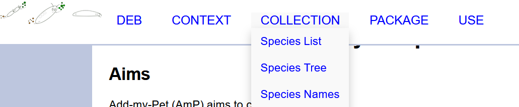
You can navigate the collection via the dropdown menu collection and choosing species list, species tree or species names.
From there access the species of your choice.
See screen shot here below.
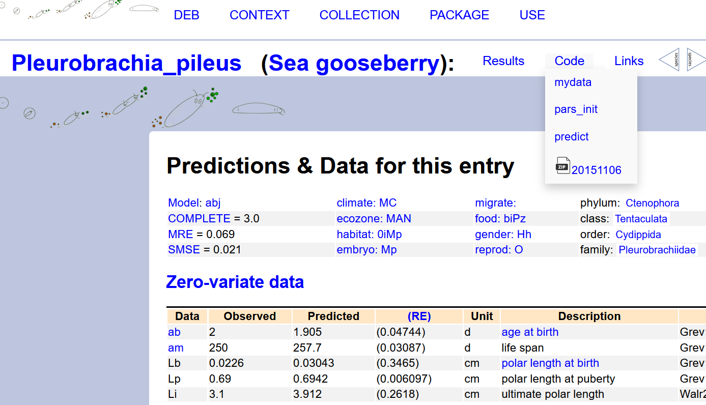
 Next, once you are in the species specific page of your choice, you can dowload its mydata-file via the code dropdown menu.
See screenshot here below.
Next, once you are in the species specific page of your choice, you can dowload its mydata-file via the code dropdown menu.
See screenshot here below.
 If you are not interested to access the mydata-file for a species via the website, you may do this via typing an appropriate query into your Matlab console.
Function
If you are not interested to access the mydata-file for a species via the website, you may do this via typing an appropriate query into your Matlab console.
Function get_data does the same and deletes the local mydata-file after running it:
vars_pull(get_data('Daphnia_magna'))
mydata_Daphnia_magna.m directly to variables in your work directory.
The rest of this guidance page focusses on meta-data and derived data: parameters, meta-parameters and implied traits.
All functions that analyse data do so by reading information contained in allStat.mat via two functions:
read_allStat(reads data from the entire collection)read_stat(same as previous function except that user specifies in the first argument which species to read data for)
t_g is given at T_typical (aka body temperature). Convert the value to the reference temperature T_ref with the following code:
		[var, nm, units, label] = read_allStat('t_g','c_T');
		tg_Tref = var(:,1).*var(:,2);
prt_tab({nm, tg_Tref},{'name',[label{1}, ', ', units{1,1}]})
NaN (Not-a-Number).
The function can also be used to write an csv or Excell file.
Here is some example code enabling a user to find all entries that have model std:
[model, nms] = read_allStat('model'); nms(strcmp('std', model))
Some further examples of code to try:
		prt_tab({select('Daphniidae'),read_stat(select('Daphniidae'),{'p_M','R_i'})},{'species','[p_M]','R_i'}) % outputs a table with selected properties of selected species to html format
		prt_tab({select('Daphniidae'),read_stat(select('Daphniidae'),{'p_M','R_i'})}) % outputs same table without headers
		read_stat(select('Daphniidae'),{'p_M','R_i'}) % outputs to matlab console, no species names printed, just numbers
		read_stat('Daphnia_magna','p_M') % outputs spec maintenance for D. magna to console
Subfields ecoCode in allStat specifies climate, ecozone, habitat, embryo environment,
migration/torpor, food, gender and reproduction mode for each entry.
The codes are explained in AmPeco, assigned in the mydata-files.
All functions that analyse eco-codes use function
read_allEco or read_eco.
prt_report_my_pet can be used to get parameters and
implied traits for specific entries.
prt_report_my_pet('Daphnia_magna'); will open an htlm-page in your browser, that allows for searching of traits and has the option "short/medium/long/pars"
to reduce the length of the table.
The "implied traits"-pages on the AmP-website present a subset of the shown list (but has no searching facilities).
The function reads parameters in allStat and specifies scaled functional response and temperature for each trait.
The function is also used during the parameter estimation procedure for entries that are not yet in the collection with
estim_options('results_output', 4); in the run_my_pet file.
In this application the data is not read from allStat, but computed from parameters, using the same routines that were used to obtain allStat.
This is handy for checking that a particular parameter combination is yes or no realistic.
With estim_options('results_output', 5);, related species are included in the report to compare parameters and implied traits.
These related species in the collection are identified with function clade (see below), and if two or more related species are found,
color coding is applied to highlight eccentricity of values.
The selection of "related" species can be specified in the run-file explicitly by declaring global variable refPets and filling it with a cell-string of AmP-species names.
Variable refPets is only used if results_output level is 5 or higher.
gallery_png writes and opens fig_png.html that links all png-files
in the AmP-collection for a specified taxon, or cell-string of entries.
This can be handy for selecting entries.
If the (first) input is missing, all entries are selected, and a very large fig_png-file results.
Taxonomic tree: lists-of-lists
Entries are organised according to the taxonomic position of the taxa that they represent. This position is determined in lists-of-lists, stored inAmPtool/taxa; the taxonomic info in the mydata-files is only used for presentation in
the species-list and
for the default value of the water content by function get_d_V
and the default nitrogen waste by function get_N_waste.
Further it is used to identify the phylum, class and order names in the function list_taxa (see below).
A list is a simple text-file.
Several functions link these lists into a tree.
The tree has a root, here called Animalia, nodes, which are names of taxa, and leaves, which are names of entries.
Most entries represent a species, but some species have multiple entries, such as geographical races.
Each node once occurs in a list and once as name of a list; the root only occurs once as a name of a list.
All entry (= leaf) names have an underscore in their name, while no node has an underscore.
The last node (= list name) in tree-branches only contains leaves and is a genus, which is part of the name of the entries it contains.
No other node contains leaves.
Function list_taxa returns a list of all nodes and (optionally) leaves; you can also extract genera, families or phyla only.
list_taxa('Deuterostomata',4) returns a list of all deuterostome families in the collection and list_taxa('',7) a list of all animal phyla.
Print-and-open an html-table with numbers of AmP entries with e.g. get_n(list_taxa('Carnivora',4)).
The species-sequence on the AmP web-pages species-list and
species-tree is composed from this tree.
Compose your own interactive tree with treeview_taxa, with any node as root,
including pictures on the nodes and links on the leaves, if you are web-connected, e.g. treeview_taxa('Crustacea').
It can also show the distribution of some statistic, i.e. parameter or implied trait, among the taxa in the (small) tree with background colour gradients.
This statistic can be symbolic, with a name matching some field in allStat, or numeric, e.g. computed from values in allStat:
treeview_taxa('Cladocera', 'kap').
Function select_taxon let you choose a taxon from a list of all possibilities.
If you are not sure about the possible nodes, or want to avoid spelling errors:
treeview_taxa(select_taxon('Arthropoda', 5))
The tree can be read in the direction from leaves to root with the function lineage,
and in the direction from root to leaves with the function pedigree.
The default input of pedigree is the root Animalia, but can also be any node, which becomes the root of the output-tree.
The (character) string produced by pedigree can directly be printed to the screen, which is useful for small trees.
The tree can be used to identify useful taxa for analysis.
The function galleryAmP('Cephalopoda') composes a gallery of pictures for taxon Cephalopoda (in this case);
clicking on a picture opens the tree at the seleted taxon.
A few taxa have a special status.
Reptilia and Sarcopterygii are used in mydata, will not occur in lineage, but can be used in select.
Pisces is not used in mydata, will not occur in lineage, but can be used in select.
Selection of entries
AmP has a number of select-functions, i.e. functions that either return a cell-string of entry names or a vector of booleans (i.e. of the true/false type). These functions scan the whole collection and select entries that comply to a variety of specified criteria.Selection on taxonomy
A motivation for this type of selection could be to study evolutionary adaptations of parameter values and implied traits. Inclusion of very unrelated species in plots of traits typically results in a blurr that is not very informative. Selection of entries via the tree is done with the functionsselect and select_01.
Select returns a cell-string with names of selected entries, select_01 a vector of booleans and a cell-string with the names of all entries.
Notice that allStat and the lists-of-lists change continuously, so do the results of select and select_01.
Function clade finds the lowest taxon (= node in the tree) that contains a set of specified taxa,
and all its members that exist in the collection.
It combines functions lineage and pedigree and can also be used to find the closest relatives of a single specified taxon.
If a species is not found in the AmP collection, it searches the Catalog of Life and
the Taxonomicon for lineages,
with functions lineage_CoL and lineage_Taxo and
presents the AmP species that are most related.
Print (compound) parameters or statistics of selected entries to screen with prtStat, or,
including the tree-structure, with pedigree.
Use clade to select related entries and catenate with prtStat by e.g.
prtStat(clade('Lemmus_trimucronatus'),'p_M');
Include the tree as well by e.g.
[~, taxon] = clade('Lemmus_trimucronatus'); pedigree(taxon,'p_M')Selection on eco-codes
A motivation for this type of selection could be to study ecological adaptations of parameter values. Selection on eco-codes is done with function select_eco. It allows selection for a single variable, and multiple codes in OR mode. Selection of all (terrestrial and marine) Antarctic species is done withselect_eco('ecozone', {'MS','TS'}).
Apart from the names of the entries, it returns selection identifiers (booleans) for the whole collection, allowing to combine the result with multiple calls to this function.
For example all species in the collection that eat invertebrates (in some stage) and occur in the North-Atlantic are found with:
[nm, s1]=select_eco('food',{'Ci'}); [nm,s2]=select_eco('ecozone',{'MAN'}); nm=select; nm(s1&s2).
While food-code Cim selects for feeding on molluscs, entries with code Ci will not be selected, but some of them might eat molluscs as well.
In reverse, entries with code Cim will be selected if Ci is specified, due to the hierarchical nature of the coding system.
Codes for one particular entry my_pet can be extracted with function read_stat:
eco = read_stat({my_pet}, 'ecoCode'); eco{1}.
Possible variables and codes are given on the AmP ecology page.
Although the codes for food and habitat have stage-identifiers, they are presently not used in select_eco.
Print, e.g. the value of reproduction efficiency kap_R for all entries that are simultaneous hermaphrodite:
prtStat(select_eco('gender','Hh'),'kap_R');Selection on data types that were used for estimation
A motivation for this type of selection could be to study effects of data combinations on the estimation process. Entries with a particular combination of zero-variate and uni-variate data can be selected with function select_data. This selection can be restricted to particular typified models, which can be handy for preparing a predict-file for a new species, and for linking parameter values to source data types. The Matlab expressionprtStat(select_data({'t-Le','Wwb'},'std'),'v');Selection on strings in mydata and predict files
A motivation for this type of selection could be the question 'which entries have a changing (scaled) function response in time' and which of these entries have males and females with different parameters)? The answer involvesselect_predict, using the knowlegde that such predict files make use of
the string 'f = spline1(t, tf)' and 'male', respectively.
The required code is
[species, nm] = select_predict('f = spline1(t, tf)'); select_predict(nm, 'males')select_predict is absent in the first call (so 'Animalia' is assumed), but present in the second call.
Similarly, select_mydata can be used for mydata files, e.g. to search for particular authors in references.
Selection in general
A general multi-step way of selecting entries on the basis of a variety of criteria is, e.g. mammals that have aCOMPLETE score larger than 2.6:
[sel_M,nm]=select_01('Mammalia');sel_C=read_allStat('COMPLETE')>2.6;nm=nm(sel_M&sel_C)pM_v=read_stat(nm,'p_M','v') with:
Hfig=figure(1);plot(pM_v(:,1),pM_v(:,2),'or');.
See entry names by clicking on points in this figure with:
h=datacursormode(Hfig);h.UpdateFcn=@(obj,event_obj)xylabels(obj,event_obj,nm,pM_v);datacursormode on.
Select terrestrial Arthropods with [sel_A nm]=select_01('Arthropoda'); [~,sel_T]=select_eco('habitat','T'); nm(sel_A&sel_T).
(Notice that the stage-codes are not used in the selection, and that the result includes species that combine terrestrial with aquatic life stages.)
Select North American freshwater fish with
	[sel_P,nm]=select_01('Pisces');
	[~,sel_TH]=select_eco('ecozone','TH');
	[~,sel_THp]=select_eco('ecozone','THp');
        nm=nm(sel_P&sel_TH&~sel_THp)
TH, comprises the palearctic, THp, and the nearctic, THn.
Selection for nearctic species would miss the holarctic ones.
Although Pisces is not a clade (= natural taxon), so not a node in the tree, it can serve handy functions.)
Since the selection-booleans that result from select, select_eco and select_data all have the same sequence of entries,
the three types of selection can be combined.
select_mydata and select_predict
have selection-booleans as third output, which can be used for more advanced and/or conditions.
The code for answering the question 'which birds have males different from females or varying body temperature during development' could read
	 [x,nm,sel_m]=select_predict('Aves','male');
	 [x,nm,sel_T]=select_predict(nm,'del_l');
	 nm(sel_m|sel_T)
To get all names of entries that have model hax, you can write
[model, nm] = read_allStat('model'); nm_hax = nm(strcmp(model,'hax'))
Legend exploits selections
Spotting patterns in (functions of) parameters of entries starts with plot function shstat (see below; the name stands for "show statistics"), which has inputs data and legend (and optional further inputs).
A (marker) legend is a (n,2)-array of cells specifiying markers and taxa (= nodes and/or leaves as character strings) or eco-codes (as cell strings).
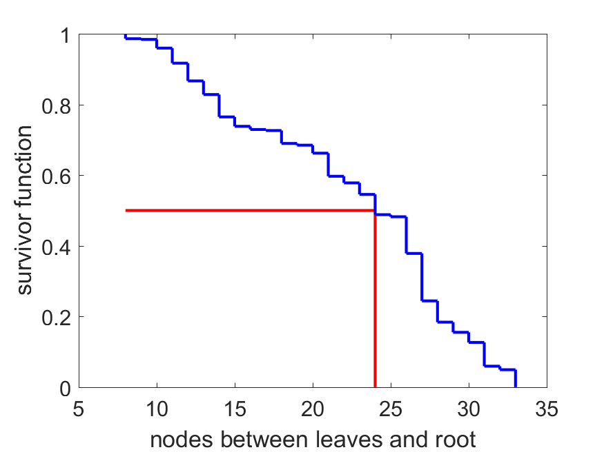
A line legend, called llegend, does this for lines and taxa; it is used for 1-variate data, e.g. survivor functions.
Several legends are available as input-free functions that output the required cell-array,
such as legend_RSED and legend_fish.
Customised legends can be composed by functions
select_legend, select_legend_eco and
select_llegend.
Alternatively, you can copy the contents of a template, such as legend_RSED, and edit it.
The result does not need to be a function; it can be just a variable in some function.
The choice of possible taxa is restricted to the ones present in the lists-of-lists and that of eco-codes to the codes mentioned in
AmPeco.
Legends can be shown in a figure with DEBtool_M functions shlegend and
shllegend.
Please notice that the sequence of rows of marker legends matters, see shstat;
this is a consequence of the fact that one taxon can contain another one.
Here are three examples of legends that are set in code:
       legend = {...
         {'o', 8, 3, [0 0 0], [1 1 1]}, 'Cyclostomata'; ...
         {'o', 8, 3, [0 0 1], [1 1 1]}, 'Chondrichthyes'; ....
         {'o', 8, 3, [1 0 0], [1 1 1]}, 'Actinopterygii'; ....
         {'o', 8, 3, [1 0 1], [1 1 1]}, 'Latimeria'; ....
         {'o', 8, 3, [0.5 0 0.5], [1 1 1]}, 'Dipnoi'; ....
         {'.', 8, 3, [0 0 0], [1 1 1]}, 'vertebrata'; ....
       };

       llegend = {...
         {'-', 2, [0 0 0]}, 'Cyclostomata'; ....
         {'-', 2, [0 0 1]}, 'Chondrichthyes'; ....
         {'-', 2, [1 0 0]}, 'Actinopterygii'; ....
         {'-', 2, [1 0 1]}, 'Latimeria'; ....
         {'-', 2, [0.5 0 0.5]}, 'Dipnoi'; ....
       };

       llegend_CAA = {...
         {'-', 2, [0 0 0]}, 'Animalia'; ....
         {'-', 2, [0 1 0]}, 'Chondrichthyes'; ....
         {'-', 2, [1 0 0]}, 'Actinopterygii'; ....
       };
Spotting patterns in data with legend

Function shstat can be used in symbolic mode for 1-, 2- and 3-variate data, as given in allStat.
In this mode, shstat is using read_allStat to read in allStat;
a large number of symbols for (functions of) parameters is available, following DEB notation.
Functions of parameters that do not depend on food, called compound parameters, were computed with DEBtool_M function
parscomp_st,
and that do with
statistics_st.
These functions briefly describe the various variables, which are presented in context in the DEB book.
Function shstat can also be used in numerical mode in the case that computations are required,
e.g. for functions of parameters that are not already in allStat.
In this case, shstat does not read in allStat, but still links data to entries via legends.
An ecocode legend is recognized by the cell-strings in the second column, while taxa appear as character-strings.
Markers in plots can be clicked to show the names of the corresponding entries.
The script mydata_shstat gives examples of use of shstat and
shows how items can be added to figures that have been produced by shstat.
If markers in 3D plots do not have color specifications, the third variable is used to set the colors in the lava color scheme, see
shcolor_lava, using
color_lava.
Get a rapid overview of distributions of a number of (compound) parameters or statistics for selected taxa with compare_taxa.
Plot (compound) parameters or statistics as function of normalised taxonomic distance with (computation-time intensive) function shstat_taxa.
An example of the use of presentation tools of AmPtool is given in mydata_Cephalopoda.
Several papers in the section Patterns in parameter values of the DEBpapers-page
point to supporting information (SI) with code to create the figures of these papers as examples of the presentation capabilities of AmPtool.
Plotting with entries that are not (yet) in the AmP collection
Suppose that you have an entry locally, i.e. the fileresults_my_pet.mat that is created by estim_pars, but this entry is not yet in the collection and
you want to see how the implied traits relate to the ones in the collection.
Three actions need to take place in preparation
- the species needs to be added to the lists-of-lists in
AmPtool/taxa. This means that the genus of your entry needs to be added to its family-list, if it is not already there, and your species needs to be added to the genus-list. If the genus is also not already present, a new list for that genus needs to be created with your entry-name, which must have an underscore and no spaces. Some large families have subfamilies, or even tribes, meaning that your genus might need to be added there, rather than in the family-list. Likewise, if the family is not already in the lists-of-lists, it should be added to its order-list and a new family list should be created. Each taxon above the species-level should occur exactly 2 times in the lists-of-lists, once as member of a higher taxon and once as name of its own list. Check the successful addition to the lists-of-lists with functionpedigree. Notice that these edits go lost if you reloadAmPtoolfrom GitHub. - your entry needs to be added to the local structures
allStatandpopStat. This can be done by runningaddEntryLoc. Make sure that your entry is added to the lists-of-lists before you runaddEntryLocand that the path to AmPdata has been set within Matlab. The addition to allStat and popStat is done with the default temperature for allStat, namelyT_typical, and food is abundant,f=1; Use the entry-specific temperature correction factor,c_Tand the temperature parameters, for other temperatures. Check the successful addition toallStatwithload allStat; allStat.my_pet, wheremy_petis replaced by the name of your entry. Notice that these edits go lost if you re-downloadAmPdatafrom the AmP-website, whileAmPdatais changing frequently. - you possibly want to edit a legend to recognize your species in plots.
Allthough the example templates like
legend_RSEDare functions that fill a variable, it can be a variable directly. Check the proper formulation of a legend withshlegend. Notice that you can always click on a point in a figure that is produced byshstatto see the name of the corresponding species.
shstat, read_stat, read_popStat and read_allStat assume that
the leaves (= endpoints, so the entry-names) of the lists-of-lists exactly correspond with the fields of allStat and popStat.
Plotting trajectories of states and traits
The functionsimu_my_pet
produces plots of trajectories of the state of an individual and some traits, from start of development to death by aging, in a possibly dynamic environment
(in terms of temperature and food).
It extracts the required parameters from the AmP via allStat, but also via results_my_pet.mat.
The latter use allows to plot trajectories for entries that are not (yet) in the collection (see previous subsection), or to modify parameters.
Here is example code for choosing variable temperature and variable food and then calling simu_my_pet for a species in AmP:
	t = linspace(0, 10*365, 5000); % d, time vector
	tT_0 = 90; % d, phase shift for sinusoidal function for temperature
	tf_0 = 250; % d, phase shift for sinusoidal function for food
	T = C2K(21) + 6 * sin(2 * pi * (t + tT_0)/ 365); % K, sinusoidal function for temperature
	f = 0.8 + 0.2 * sin(2 * pi * (t + tf_0)/ 365); % -, sunusoidal function for food level
	tT =[t',T']; % d, K, temperature matrix
	tf =[t',f']; % d, -, food level matrix
	simu_my_pet('Megalobulimus_mogianensis', tT ,tf)
See also the DEBsea Shiny apps in the PACKAGE menu bar.
The DEBsea Shiny apps can be used for simulating the DEB model given real environmental conditions (temperature from NOAA given time and location) and which are run on the server of Melbourne University.
Linked websites
Function get_links can be used for the addresses of all websites, as specified in the mydata-file for that species; typeget_links('Homo_sapiens', 1) to open them all in your system-browser.
Function get_id does something similar, but gets the identifiers from the web, not from the AmP collection.
The species name can be any valid one, known in CoL.
This function might make use of get_synonym;
it first tries the corresponding accepted name in CoL, then the name that the user provided and finally an alternative name, if provided by CoL.
If the species cannot be found, it tries the genus for several websites.
Notice that several websites have problems with finding species due to the inclusion of the subgenus in the name (of some genera).
E.g. CoL cannot find 'Daphnia magna', only 'Daphnia (Ctenodaphnia) magna'.
The id-table gives an overview of all id's for all entries and supported websites. Click on a web-site column-header to let it disappear, and on the entry-header to let it re-appear.
Distances between species: Multi-dimensional scaling
Function dist_taxa computes the taxonomic distances between species (it is computational intensive), and dist_traits for trait-distances. A trait is here any parameter or function of parameters, as present inallStat, and the set of traits can be arbitrarily large, with optional weights.
The distance-measure is the symmetric bounded or unbouded loss function.
Tools for MultiDimensional Scaling (MDS) can be used to further analyse these distance matrices; Matlab has, for instance, function cmdscale for this purpose.
The script AmPtool/mydata_mds_Carnivora gives an example for a selection of traits for the Carnivora,
showing the use of shstat in this context and
connecting clades members with connect_subclade.